You are viewing the static version of the notebook, you can get the code (GitHub) or run it in colab

You can also do the quizzes

Module 2: PyTorch tensors and automatic differentiation

Video timestamp

import matplotlib.pyplot as plt
%matplotlib inline
import torch
import numpy as np

torch.__version__

Tensors are used to encode the signal to process, but also the internal states and parameters of models.

Manipulating data through this constrained structure allows to use CPUs and GPUs at peak performance.

Construct a 3x5 matrix, uninitialized:

x = torch.empty(3,5)
print(x.dtype)
print(x)

If you got an error this stackoverflow link might be useful...

x = torch.randn(3,5)
print(x)

print(x.size())

torch.Size is in fact a tuple, so it supports the same operations.

Video timestamp

x.size()[1]

x.size() == (3,5)

Bridge to numpy

Video timestamp

y = x.numpy()
print(y)

a = np.ones(5)
b = torch.from_numpy(a)
print(a.dtype)
print(b)

c = b.long()
print(c.dtype, c)
print(b.dtype, b)

xr = torch.randn(3, 5)
print(xr.dtype, xr)

resb = xr + b
resb

resc = xr + c
resc

Be careful with types!

resb == resc

torch.set_printoptions(precision=10)

resb[0,1]

resc[0,1]

resc[0,1].dtype

xr[0,1]

torch.set_printoptions(precision=4)

Broadcasting

Video timestamp

Broadcasting automagically expands dimensions by replicating coefficients, when it is necessary to perform operations.

1. If one of the tensors has fewer dimensions than the other, it is reshaped by adding as many dimensions of size 1 as necessary in the front; then

2. for every mismatch, if one of the two tensor is of size one, it is expanded along this axis by replicating coefficients.

If there is a tensor size mismatch for one of the dimension and neither of them is one, the operation fails.

A = torch.tensor([[1.], [2.], [3.], [4.]])
print(A.size())
B = torch.tensor([[5., -5., 5., -5., 5.]])
print(B.size())
C = A + B

C

The original (column-)vector

\[\begin{array}{rcl} A = \left( \begin{array}{c} 1\\ 2\\ 3\\ 4\\ \end{array}\right) \end{array}\]

is transformed into the matrix

\[\begin{array}{rcl} A = \left( \begin{array}{ccccc} 1&1&1&1&1\\ 2&2&2&2&2\\ 3&3&3&3&3\\ 4&4&4&4&4 \end{array}\right) \end{array}\]

and the original (row-)vector

\[\begin{array}{rcl} C = (5,-5,5,-5,5) \end{array}\]

is transformed into the matrix

\[\begin{array}{rcl} C = \left( \begin{array}{ccccc} 5&-5&5&-5&5\\ 5&-5&5&-5&5\\ 5&-5&5&-5&5\\ 5&-5&5&-5&5 \end{array}\right) \end{array}\]

so that summing these matrices gives:

\[\begin{array}{rcl} A+C = \left( \begin{array}{ccccc} 6&-4&6&-4&6\\ 7&-3&7&-3&7\\ 8&-2&8&-2&8\\ 9&-1&9&-1&9 \end{array}\right) \end{array}\]

In-place modification

Video timestamp

x

xr

print(x+xr)

x.add_(xr)
print(x)

Any operation that mutates a tensor in-place is post-fixed with an _

For example: x.fill_(y), x.t_(), will change x.

print(x.t())

x.t_()
print(x)

Shared memory

Video timestamp

Also be careful, changing the torch tensor modify the numpy array and vice-versa...

This is explained in the PyTorch documentation here: The returned tensor by torch.from_numpy and ndarray share the same memory. Modifications to the tensor will be reflected in the ndarray and vice versa.

a = np.ones(5)
b = torch.from_numpy(a)
print(b)

a[2] = 0
print(b)

b[3] = 5
print(a)

Cuda

Video timestamp

torch.cuda.is_available()

#device = torch.device('cpu')
device = torch.device('cuda') # Uncomment this to run on GPU

x.device

# let us run this cell only if CUDA is available
# We will use ``torch.device`` objects to move tensors in and out of GPU
if torch.cuda.is_available():
    y = torch.ones_like(x, device=device)  # directly create a tensor on GPU
    x = x.to(device)                       # or just use strings ``.to("cuda")``
    z = x + y
    print(z,z.type())
    print(z.to("cpu", torch.double))       # ``.to`` can also change dtype together!

x = torch.randn(1)
x = x.to(device)

x.device

# the following line is only useful if CUDA is available
x = x.data
print(x)
print(x.item())
print(x.cpu().numpy())

Simple interfaces to standard image data-bases

Video timestamp

An example, the CIFAR10 dataset.

import torchvision

data_dir = 'content/data'

cifar = torchvision.datasets.CIFAR10(data_dir, train = True, download = True)
cifar.data.shape

Documentation about the permute operation.

x = torch.from_numpy(cifar.data).permute(0,3,1,2).float()
x = x / 255
print(x.type(), x.size(), x.min().item(), x.max().item())

Documentation about the narrow(input, dim, start, length) operation.

# Narrows to the first images, converts to float
x = torch.narrow(x, 0, 0, 48)

x.shape

# Showing images
def show(img):
    npimg = img.numpy()
    plt.figure(figsize=(20,10))
    plt.imshow(np.transpose(npimg, (1,2,0)), interpolation='nearest')
    
show(torchvision.utils.make_grid(x, nrow = 12))

# Kills the green and blue channels
x.narrow(1, 1, 2).fill_(0)
show(torchvision.utils.make_grid(x, nrow = 12))

Autograd: automatic differentiation

Video timestamp

When executing tensor operations, PyTorch can automatically construct on-the-fly the graph of operations to compute the gradient of any quantity with respect to any tensor involved.

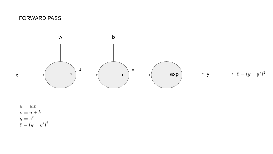
To be more concrete, we introduce the following example: we consider parameters \(w\in \mathbb{R}\) and \(b\in \mathbb{R}\) with the corresponding function:

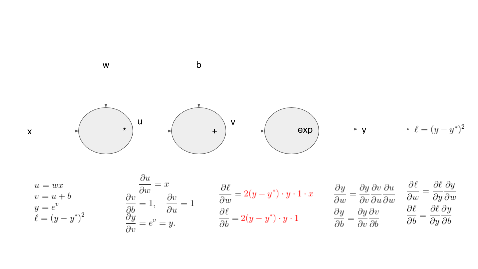
Our goal here, will be to compute the following partial derivatives:

The reason for doing this will be clear when you will solve the practicals for this lesson!

You can decompose this function as a composition of basic operations. This is call the forward pass on the graph of operations.

Let say we start with our model in numpy:

w = np.array([0.5])
b = np.array([2])
xx = np.array([0.5])#np.arange(0,1.5,.5)

transform these into tensor:

xx_t = torch.from_numpy(xx)
w_t = torch.from_numpy(w)
b_t = torch.from_numpy(b)

Video timestamp

A tensor has a Boolean field requires_grad, set to False by default, which states if PyTorch should build the graph of operations so that gradients with respect to it can be computed.

w_t.requires_grad

We want to take derivative with respect to \(w\) so we change this value:

w_t.requires_grad_(True)

We want to do the same thing for \(b\) but the following line will produce an error!

b_t.requires_grad_(True)

Reading the error message should allow you to correct the mistake!

dtype = torch.float64

b_t = b_t.type(dtype)

b_t.requires_grad_(True)

Video timestamp

We now compute the function:

def fun(x,ystar):
    y = torch.exp(w_t*x+b_t)
    print(y)
    return torch.sum((y-ystar)**2)

ystar_t = torch.randn_like(xx_t)
l_t = fun(xx_t,ystar_t)

l_t

l_t.requires_grad

After the computation is finished, i.e. forward pass, you can call .backward() and have all the gradients computed automatically.

print(w_t.grad)

l_t.backward()

print(w_t.grad)
print(b_t.grad)

Video timestamp

Let's try to understand these numbers...

yy_t = torch.exp(w_t*xx_t+b_t)
print(torch.sum(2*(yy_t-ystar_t)*yy_t*xx_t))
print(torch.sum(2*(yy_t-ystar_t)*yy_t))

tensor.backward() accumulates the gradients in the grad fields of tensors.

l_t = fun(xx_t,ystar_t)
l_t.backward()

print(w_t.grad)
print(b_t.grad)

By default, backward deletes the computational graph when it is used so that you will get an error below:

l_t.backward()

# Manually zero the gradients
w_t.grad.data.zero_()
b_t.grad.data.zero_()
l_t = fun(xx_t,ystar_t)
l_t.backward(retain_graph=True)
l_t.backward()
print(w_t.grad)
print(b_t.grad)

The gradients must be set to zero manually. Otherwise they will cumulate across several .backward() calls. This accumulating behavior is desirable in particular to compute the gradient of a loss summed over several “mini-batches,” or the gradient of a sum of losses.