![]()
You are viewing the static version of the notebook, you can get the code (GitHub) or run it in colab
To illustrate the Deep Learning pipeline seen in Module 1, we are going to use a pretrained model to enter the Dogs vs Cats competition at Kaggle.
There are 25,000 labelled dog and cat photos available for training, and 12,500 in the test set that we have to try to label for this competition. According to the Kaggle web-site, when this competition was launched (end of 2013): "State of the art: The current literature suggests machine classifiers can score above 80% accuracy on this task". So if you can beat 80%, then you will be at the cutting edge as of 2013!
import numpy as np
import matplotlib.pyplot as plt
import os
import torch
import torch.nn as nn
import torchvision
from torchvision import models,transforms,datasets
import time
%matplotlib inline
Here you see that the latest version of PyTorch is installed by default.
torch.__version__import sys
sys.versionCheck if GPU is available and if not change the runtime.
device = torch.device("cuda:0" if torch.cuda.is_available() else "cpu")

print('Using gpu: %s ' % torch.cuda.is_available())You can download the full dataset from Kaggle directly.
Alternatively, Jeremy Howard (fast.ai) provides a direct link to the catvsdogs dataset. He's separated the cats and dogs into separate folders and created a validation folder as well.
For test purpose (or if you run on cpu), you should use the (small) sample directory.
%mkdir data
# the following line should be modified if you run the notebook on your computer
# change directory to data where you will store the dataset
%cd /content/data/
!wget http://files.fast.ai/data/examples/dogscats.tgz
!tar -zxvf dogscats.tgz%ls%cd dogscats/
%lsThe structure of the sub-folders inside the folder dogscats will be important for what follows:
.
├── test1 # contains 12500 images of cats and dogs
├── train
|   └── cats # contains 11500 images of cats
|   └── dogs # contains 11500 images of dogs
├── valid
|   └── cats # contains 1000 images of cats
|   └── dogs # contains 1000 images of dogs
├── sample
|   └── train
|       └── cats # contains 8 images of cats
|       └── dogs # contains 8 images of dogs
|   └── valid
|       └── cats # contains 4 images of cats
|       └── dogs # contains 4 images of dogs
├── models # empty folder
You see that the 12 500 images of the test are in the test1 sub-folder; the dataset of 25 000 labelled images has been split into a train set and a validation set.
The sub-folder sample is here only to make sure the code is running properly on a very small dataset.
%cd ..Below, we give the path where the data is stored. If you are running this code on your computer, you should modifiy this cell.
data_dir = '/content/data/dogscats'datasets is a class of the torchvision| package (see torchvision.datasets) and deals with data loading. It integrates a multi-threaded loader that fetches images from the disk, groups them in mini-batches and serves them continously to the GPU right after each forward/backward pass through the network.
Images needs a bit of preparation before passing them throught the network. They need to have all the same size plus some extra formatting done below by the normalize transform (explained later).
normalize = transforms.Normalize(mean=[0.485, 0.456, 0.406], std=[0.229, 0.224, 0.225])

imagenet_format = transforms.Compose([
                transforms.CenterCrop(224),
                transforms.ToTensor(),
                normalize,
            ])
dsets = {x: datasets.ImageFolder(os.path.join(data_dir, x), imagenet_format)
for x in ['train', 'valid']}os.path.join(data_dir,'train')Interactive help on jupyter notebook thanks to ?
?datasets.ImageFolderWe see that datasets.ImageFolder has attributes: classes, classtoidx, imgs.
Let see what they are?
dsets['train'].classesThe name of the classes are directly inferred from the structure of the folder:
├── train
|   └── cats
| └── dogsdsets['train'].class_to_idxThe label 0 will correspond to cats and 1 to dogs.
Below, you see that the first 5 imgs are pairs (locationofthe_image, label):
dsets['train'].imgs[:5]dset_sizes = {x: len(dsets[x]) for x in ['train', 'valid']}
dset_sizesAs expected we have 23 000 images in the training set and 2 000 in the validation set.
Below, we store the classes in the variable dset_classes:
dset_classes = dsets['train'].classesThe torchvision packages allows complex pre-processing/transforms of the input data (e.g. normalization, cropping, flipping, jittering). A sequence of transforms can be grouped in a pipeline with the help of the torchvision.transforms.Compose function, see torchvision.transforms
The magic help ? allows you to retrieve function you defined and forgot!
?imagenet_formatWhere is this normalization coming from?
As explained in the PyTorch doc, you will use a pretrained model. All pre-trained models expect input images normalized in the same way, i.e. mini-batches of 3-channel RGB images of shape (3 x H x W), where H and W are expected to be at least 224. The images have to be loaded in to a range of [0, 1] and then normalized using mean = [0.485, 0.456, 0.406] and std = [0.229, 0.224, 0.225].
loader_train = torch.utils.data.DataLoader(dsets['train'], batch_size=64, shuffle=True, num_workers=6)?torch.utils.data.DataLoaderloader_valid = torch.utils.data.DataLoader(dsets['valid'], batch_size=5, shuffle=False, num_workers=6)Try to understand what the following cell is doing?
count = 1
for data in loader_valid:
    print(count, end=',')
    if count == 1:
        inputs_try,labels_try = data
count +=1labels_tryinputs_try.shapeGot it: the validation dataset contains 2 000 images, hence this is 400 batches of size 5. labels_try contains the labels of the first batch and inputs_try the images of the first batch.
What is an image for your computer?
inputs_try[0]A 3-channel RGB image is of shape (3 x H x W). Note that entries can be negative because of the normalization.
A small function to display images:
def imshow(inp, title=None):
#   Imshow for Tensor.
    inp = inp.numpy().transpose((1, 2, 0))
    mean = np.array([0.485, 0.456, 0.406])
    std = np.array([0.229, 0.224, 0.225])
    inp = np.clip(std * inp + mean, 0,1)
    plt.imshow(inp)
    if title is not None:
        plt.title(title)
# Make a grid from batch from the validation data
out = torchvision.utils.make_grid(inputs_try)
imshow(out, title=[dset_classes[x] for x in labels_try])# Get a batch of training data
inputs, classes = next(iter(loader_train))
n_images = 8
# Make a grid from batch
out = torchvision.utils.make_grid(inputs[0:n_images])
imshow(out, title=[dset_classes[x] for x in classes[0:n_images]])The torchvision module comes with a zoo of popular CNN architectures which are already trained on ImageNet (1.2M training images). When called the first time, if pretrained=True the model is fetched over the internet and downloaded to ~/.torch/models. For next calls, the model will be directly read from there.
model_vgg = models.vgg16(pretrained=True)We will first use VGG Model without any modification. In order to interpret the results, we need to import the 1000 ImageNet categories, available at: https://s3.amazonaws.com/deep-learning-models/image-models/imagenetclassindex.json
!wget https://s3.amazonaws.com/deep-learning-models/image-models/imagenet_class_index.jsonimport json
fpath = '/content/data/imagenet_class_index.json'
with open(fpath) as f:
class_dict = json.load(f)
dic_imagenet = [class_dict[str(i)][1] for i in range(len(class_dict))]dic_imagenet[:4]inputs_try , labels_try = inputs_try.to(device), labels_try.to(device)
model_vgg = model_vgg.to(device)outputs_try = model_vgg(inputs_try)outputs_tryoutputs_try.shapeTo translate the outputs of the network into 'probabilities', we pass it through a Softmax function
m_softm = nn.Softmax(dim=1)
probs = m_softm(outputs_try)
vals_try,preds_try = torch.max(probs,dim=1)
Let check, that we obtain a probability!
torch.sum(probs,1)vals_tryprint([dic_imagenet[i] for i in preds_try.data])out = torchvision.utils.make_grid(inputs_try.data.cpu())
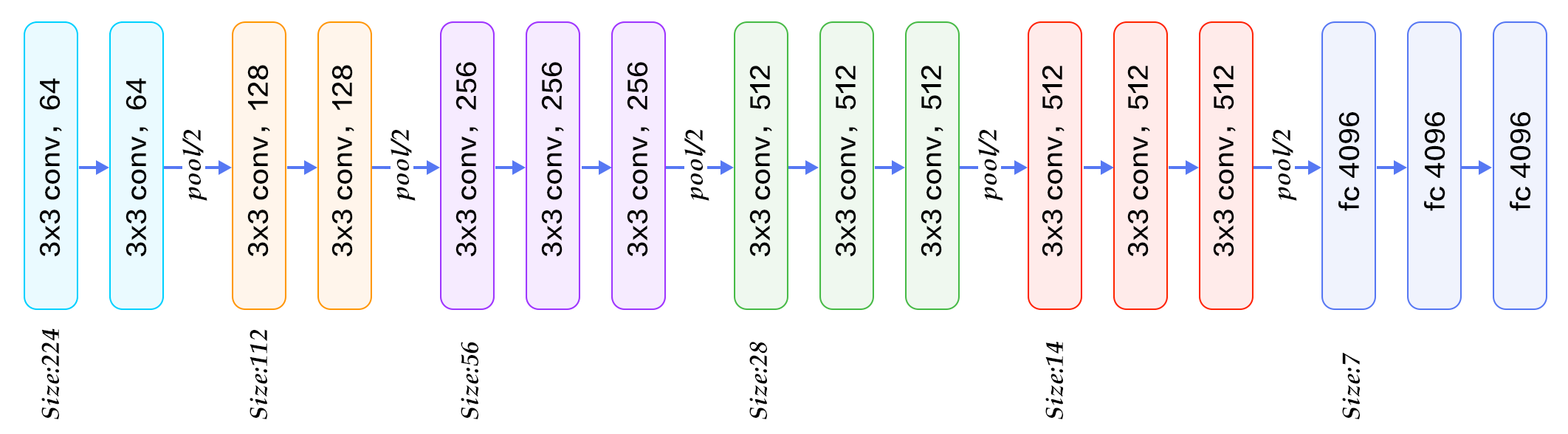
imshow(out, title=[dset_classes[x] for x in labels_try.data.cpu()])print(model_vgg)We'll learn about what these different blocks do later in the course. For now, it's enough to know that:
Convolution layers are for finding small to medium size patterns in images – analyzing the images locally
Dense (fully connected) layers are for combining patterns across an image – analyzing the images globally
Pooling layers downsample – in order to reduce image size and to improve invariance of learned features
In this practical example, our goal is to use the already trained model and just change the number of output classes. To this end we replace the last nn.Linear layer trained for 1000 classes to ones with 2 classes. In order to freeze the weights of the other layers during training, we set the field required_grad=False. In this manner no gradient will be computed for them during backprop and hence no update in the weights. Only the weights for the 2 class layer will be updated.
for param in model_vgg.parameters():
    param.requires_grad = False
model_vgg.classifier._modules['6'] = nn.Linear(4096, 2)
model_vgg.classifier._modules['7'] = torch.nn.LogSoftmax(dim = 1)
PyTorch documentation for LogSoftmax
print(model_vgg.classifier)We load the model on GPU.
model_vgg = model_vgg.to(device)PyTorch documentation for NLLLoss and the torch.optim module
criterion = nn.NLLLoss()
lr = 0.001
optimizer_vgg = torch.optim.SGD(model_vgg.classifier[6].parameters(),lr = lr)def train_model(model,dataloader,size,epochs=1,optimizer=None):
model.train()
for epoch in range(epochs):
running_loss = 0.0
running_corrects = 0
for inputs,classes in dataloader:
inputs = inputs.to(device)
classes = classes.to(device)
outputs = model(inputs)
loss = criterion(outputs,classes)
optimizer.zero_grad()
loss.backward()
optimizer.step()
_,preds = torch.max(outputs.data,1)
# statistics
running_loss += loss.data.item()
running_corrects += torch.sum(preds == classes.data)
epoch_loss = running_loss / size
epoch_acc = running_corrects.data.item() / size
print('Loss: {:.4f} Acc: {:.4f}'.format(
epoch_loss, epoch_acc))%%time
train_model(model_vgg,loader_train,size=dset_sizes['train'],epochs=2,optimizer=optimizer_vgg)def test_model(model,dataloader,size):
model.eval()
predictions = np.zeros(size)
all_classes = np.zeros(size)
all_proba = np.zeros((size,2))
i = 0
running_loss = 0.0
running_corrects = 0
for inputs,classes in dataloader:
inputs = inputs.to(device)
classes = classes.to(device)
outputs = model(inputs)
loss = criterion(outputs,classes)
_,preds = torch.max(outputs.data,1)
# statistics
running_loss += loss.data.item()
running_corrects += torch.sum(preds == classes.data)
predictions[i:i+len(classes)] = preds.to('cpu').numpy()
all_classes[i:i+len(classes)] = classes.to('cpu').numpy()
all_proba[i:i+len(classes),:] = outputs.data.to('cpu').numpy()
i += len(classes)
epoch_loss = running_loss / size
epoch_acc = running_corrects.data.item() / size
print('Loss: {:.4f} Acc: {:.4f}'.format(
epoch_loss, epoch_acc))
return predictions, all_proba, all_classespredictions, all_proba, all_classes = test_model(model_vgg,loader_valid,size=dset_sizes['valid'])# Get a batch of training data
inputs, classes = next(iter(loader_valid))
out = torchvision.utils.make_grid(inputs[0:n_images])
imshow(out, title=[dset_classes[x] for x in classes[0:n_images]])outputs = model_vgg(inputs[:n_images].to(device))
print(torch.exp(outputs))classes[:n_images]Here you are wasting a lot of time computing over and over the same quantities. Indeed, the first part of the VGG model (called features and made of convolutional layers) is frozen and never updated. Hence, we can precompute for each image in the dataset, the output of these convolutional layers as these outputs will always be the same during your training process.
This is what is done below.
x_try = model_vgg.features(inputs_try)x_try.shapeYou see that the features computed for an image is of shape 512x7x7 (above we have a batch corresponding to 5 images).
def preconvfeat(dataloader):
    conv_features = []
    labels_list = []
    for data in dataloader:
        inputs,labels = data
        inputs = inputs.to(device)
        labels = labels.to(device)

        x = model_vgg.features(inputs)
        conv_features.extend(x.data.cpu().numpy())
        labels_list.extend(labels.data.cpu().numpy())
    conv_features = np.concatenate([[feat] for feat in conv_features])
    return (conv_features,labels_list)
%%time
conv_feat_train,labels_train = preconvfeat(loader_train)conv_feat_train.shape%%time
conv_feat_valid,labels_valid = preconvfeat(loader_valid)We will not load images anymore, so we need to build our own data loader. If you do not understand the cell below, it is OK! We will come back to it in Lesson 5...
dtype=torch.float
datasetfeat_train = [[torch.from_numpy(f).type(dtype),torch.tensor(l).type(torch.long)] for (f,l) in zip(conv_feat_train,labels_train)]
datasetfeat_train = [(inputs.reshape(-1), classes) for [inputs,classes] in datasetfeat_train]
loaderfeat_train = torch.utils.data.DataLoader(datasetfeat_train, batch_size=128, shuffle=True)
%%time
train_model(model_vgg.classifier,dataloader=loaderfeat_train,size=dset_sizes['train'],epochs=50,optimizer=optimizer_vgg)datasetfeat_valid = [[torch.from_numpy(f).type(dtype),torch.tensor(l).type(torch.long)] for (f,l) in zip(conv_feat_valid,labels_valid)]
datasetfeat_valid = [(inputs.reshape(-1), classes) for [inputs,classes] in datasetfeat_valid]
loaderfeat_valid = torch.utils.data.DataLoader(datasetfeat_valid, batch_size=128, shuffle=False)predictions, all_proba, all_classes = test_model(model_vgg.classifier,dataloader=loaderfeat_valid,size=dset_sizes['valid'])Viewing model prediction (qualitative analysis)
The most important metrics for us to look at are for the validation set, since we want to check for over-fitting.
With our first model we should try to overfit before we start worrying about how to handle that - there's no point even thinking about regularization, data augmentation, etc if you're still under-fitting! (We'll be looking at these techniques after the 2 weeks break...)
As well as looking at the overall metrics, it's also a good idea to look at examples of each of:
A few correct labels at random
A few incorrect labels at random
The most correct labels of each class (ie those with highest probability that are correct)
The most incorrect labels of each class (ie those with highest probability that are incorrect)
The most uncertain labels (ie those with probability closest to 0.5).
In general, these are particularly useful for debugging problems in the model. Since our model is very simple, there may not be too much to learn at this stage...
# Number of images to view for each visualization task
n_view = 8
correct = np.where(predictions==all_classes)[0]len(correct)/dset_sizes['valid']from numpy.random import random, permutation
idx = permutation(correct)[:n_view]idxloader_correct = torch.utils.data.DataLoader([dsets['valid'][x] for x in idx],batch_size = n_view,shuffle=True)for data in loader_correct:
inputs_cor,labels_cor = data# Make a grid from batch
out = torchvision.utils.make_grid(inputs_cor)
imshow(out, title=[l.item() for l in labels_cor])from IPython.display import Image, display
for x in idx:
display(Image(filename=dsets['valid'].imgs[x][0], retina=True))incorrect = np.where(predictions!=all_classes)[0]
for x in permutation(incorrect)[:n_view]:
#print(dsets['valid'].imgs[x][1])
display(Image(filename=dsets['valid'].imgs[x][0], retina=True))#3. The images we most confident were cats, and are actually cats
correct_cats = np.where((predictions==0) & (predictions==all_classes))[0]
most_correct_cats = np.argsort(all_proba[correct_cats,1])[:n_view]for x in most_correct_cats:
display(Image(filename=dsets['valid'].imgs[correct_cats[x]][0], retina=True))#3. The images we most confident were dogs, and are actually dogs
correct_dogs = np.where((predictions==1) & (predictions==all_classes))[0]
most_correct_dogs = np.argsort(all_proba[correct_dogs,0])[:n_view]for x in most_correct_dogs:
display(Image(filename=dsets['valid'].imgs[correct_dogs[x]][0], retina=True))What did we do in the end? A simple logistic regression! If the connection is unclear, we'll explain it on a much simpler example in the next course.
We probably killed a fly with a sledge hammer!
In our case, the sledge hammer is VGG pretrained on Imagenet, a dataset containing a lot of pictures of cats and dogs. Indeed, we saw that without modification the network was able to predict dog and cat breeds. Hence it is not very surprising that the features computed by VGG are very accurate for our classification task. In the end, we need to learn only the parameters of the last linear layer, i.e. 8194 parameters (do not forget the bias ). Indeed, this can be done on CPU without any problem.
Nevertheless, this example is still instructive as it shows all the necessary steps in a deep learning project. Here we did not struggle with the learning process of a deep network, but we did all the preliminary engineering tasks: dowloading a dataset, setting up the environment to use a GPU, preparing the data, computing the features with a pretrained VGG, saving them on your drive so that you can use them for a later experiment... These steps are essential in any deep learning project and a necessary requirement before having fun playing with network architectures and understanding the learning process.
![]()