Inductive bias in GCN: a spectral perspective

author: Marc Lelarge, course: dataflowr

run the code or open it in Colab

date: April 15, 2021

Here, we focus on Graph Convolution Networks (GCN) introduced by Kipf and Welling in their paper Semi-Supervised Classification with Graph Convolutional Networks. The GCN layer is one of the simplest Graph Neural Network layer defined by:

$h_i^{(\ell+1)} = \frac{1}{d_i+1}h_i^{(\ell)}W^{(\ell)} + \sum_{j\sim i} \frac{h_j^{(\ell)}W^{(\ell)}}{\sqrt{(d_i+1)(d_j+1)}},$

where $i\sim j$ means that nodes $i$ and $j$ are neighbors in the graph $G$, $d_i$ and $d_j$ are the respective degrees of nodes $i$ and $j$ (i.e. their number of neighbors in the graph) and $h_i^{(\ell)}$ is the embedding representation of node $i$ at layer $\ell$ and $W^{(\ell)}$ is a trainable weight matrix of shape [size_input_feature, size_output_feature].

The inductive bias of a learning algorithm is the set of assumptions that the learner uses to predict outputs of given inputs that it has not encountered. For GCN, we argue that the inductive bias can be formulated as a simple spectral property of the algorithm: GCN acts as low-pass filters. This arguments follows from recent works Simplifying Graph Convolutional Networks by Wu, Souza, Zhang, Fifty, Yu, Weinberger and Revisiting Graph Neural Networks: All We Have is Low-Pass Filters by NT and Maehara.

Here we will study a very simple case and relate the inductive bias of GCN to the property of the Fiedler vector of the graph. We'll consider the more general setting in a subsequent post.

Notations

We consider undirected graphs $G=(V,E)$ with $n$ vertices denoted by $i,j \in [n]$. $i\sim j$ means that nodes $i$ and $j$ are neighbors in $G$, i.e. $\{i,j\}\in E$. We denote by $A$ its adjacency matrix and by $D$ the diagonal matrix of degrees. The vector of degrees is denoted by $d$ so that $d= A1$. The components of a vector $x\in \mathbb{R}^n$ are denoted $x_i$ but sometimes it is convenient to see the vector $x$ as a function from $V$ to $\mathbb{R}$ and use the notation $x(i)$ instead of $x_i$.

Community detection in the Karate Club

We'll start with an unsupervised problem: given one graph, find a partition of its node in communities. In this case, we make the hypothesis that individuals tend to associate and bond with similar others, which is known as homophily.

To study this problem, we will focus on the Zachary's karate club and try to recover the split of the club from the graph of connections. The pytorch-geometric library will be very convenient.

Note that GCN are not appropriate in an unsupervised setting as no learning is possible without any label on the vertices. However, this is not a problem here as we will not train the GCN! In more practical settings, GCN are used in a semi-supervised setting where a few labels are revealed for a few nodes (more on this in the section with the Cora dataset).

from torch_geometric.datasets import KarateClub

dataset = KarateClub()
print(f'Dataset: {dataset}:')
print('======================')
print(f'Number of graphs: {len(dataset)}')
print(f'Number of features: {dataset.num_features}')
print(f'Number of classes: {dataset.num_classes}')

Dataset: KarateClub():
    ======================
    Number of graphs: 1
    Number of features: 34
    Number of classes: 4

As shown above, the default number of classes (i.e. subgroups) in pytorch-geometric is 4, for simplicity, we'll focus on a partition in two groups only:

data = dataset[0] 
biclasses = [int(b) for b in ((data.y == data.y[0]) + (data.y==data.y[5]))]

We will use networkx for drawing the graph. On the picture below, the color of each node is given by its "true" class.

from torch_geometric.utils import to_networkx

G = to_networkx(data, to_undirected=True)
visualize(G, color=biclasses)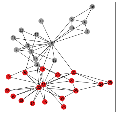

The Kernighan Lin algorithm is a heuristic algorithm for finding partitions of graphs and the results below show that it captures well our homophily assumption. Indeed the algorithm tries to minimize the number of crossing edges between the 2 communities.

c1,c2 = nx.algorithms.community.kernighan_lin_bisection(G)
classes_kl = [0 if i in c1 else 1 for i in range(34)]
visualize(G, color=classes_kl, cmap="Set2")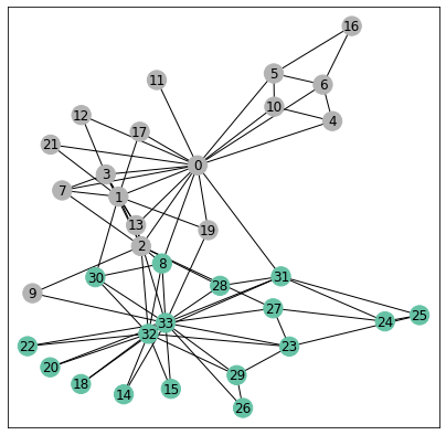

def acc(predicitions, classes):
    n_tot = len(classes)
    acc = np.sum([int(pred)==cla for pred,cla in zip(predicitions,classes)])
    return max(acc, n_tot-acc), n_tot

n_simu = 1000
all_acc = np.zeros(n_simu)
for i in range(n_simu):
    c1,c2 = nx.algorithms.community.kernighan_lin_bisection(G)
    classes_kl = [0 if i in c1 else 1 for i in range(34)]
    all_acc[i],_ = acc(classes_kl, biclasses)

The algorithm is not deterministic but performs poorly only a small fractions of the trials as shown below in the histogram for the number of correct predictions (note there are $34$ nodes in total):

bin_list = range(17,35)
_ = plt.hist(all_acc, bins=bin_list,rwidth=0.8)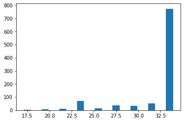

Inductive bias for GCN

To demonstrate the inductive bias for the GCN architecture, we consider a simple GCN with 3 layers and look at its performance without any training. To be more precise, the GCN takes as input the graph and outputs a vector $(x_i,y_i)\in \mathbb{R}^2$ for each node $i$.

import torch
from torch.nn import Linear
from torch_geometric.nn import GCNConv
import torch.nn.functional as F

class GCN(torch.nn.Module):
    def __init__(self):
        super(GCN, self).__init__()
        self.conv1 = GCNConv(data.num_nodes, 4)# no feature...
        self.conv2 = GCNConv(4, 4)
        self.conv3 = GCNConv(4, 2)

    def forward(self, x, edge_index):
        h = self.conv1(x, edge_index)
        h = h.tanh()
        h = self.conv2(h, edge_index)
        h = h.tanh()
        h = self.conv3(h, edge_index)
        return h

torch.manual_seed(12345)
model = GCN()
print(model)

GCN(
      (conv1): GCNConv(34, 4)
      (conv2): GCNConv(4, 4)
      (conv3): GCNConv(4, 2)
    )

Below, we draw all the points $(x_i,y_i)$ for all nodes $i$ of the graph. The vertical and horizontal lines are the medians of the $x_i$'s and $y_i$'s respectively. The colors are the true classes. We see that without any learning the points are almost separated in the lower-left and upper-right corners according to their community!

h = model(data.x, data.edge_index)
visualize(h, color=biclasses)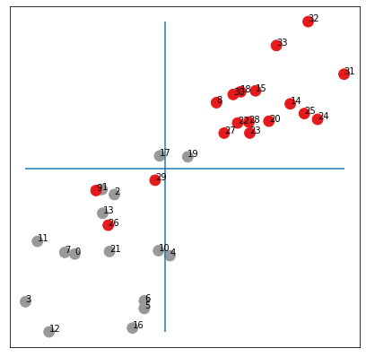

Note that by drawing the medians above, we enforce a balanced partition of the graph. Below, we draw the original graph where the color for node $i$ depends if $x_i$ is larger or smaller than the median.

color_out = color_from_vec(h[:,0])
visualize(G, color=color_out, cmap="Set2")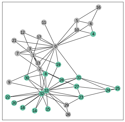

We made only a few errors without any training!

Our result might depend on the particular initialization, so we run a few more experiments below:

_ = plt.hist(all_acc, bins=bin_list,rwidth=0.8)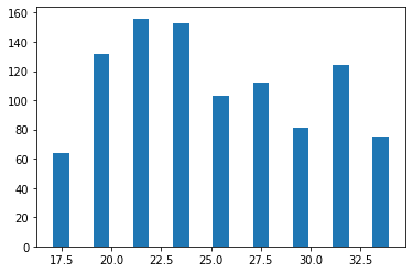

We see that on average, we have an accuracy over $24/34$ which is much better than chance!

We now explain why the GCN architecture with random initialization achieves such good results.

Spectral analysis of GCN

We start by rewriting the equation (1) in matrix form:

$h^{(\ell+1)} = S h^{(\ell)}W^{(\ell)} ,$

where the scaled adjacency matrix $S\in\mathbb{R}^{n\times n}$ is defined by $S_{ij} = \frac{1}{\sqrt{(d_i+1)(d_j+1)}}$ if $i\sim j$ or $i=j$ and $S_{ij}=0$ otherwise and $h^{(\ell)}\in \mathbb{R}^{n\times f^{(\ell)}}$ is the embedding representation of the nodes at layer $\ell$ and $W^{(\ell)}$ is the learnable weight matrix in $\mathbb{R}^{f^{(\ell)}\times f^{(\ell+1)}}$.

To simplify, we now ignore the $tanh$ non-linearities in our GCN above so that we get

$y = S^3 W^{(1)}W^{(2)}W^{(3)},$

where $W^{(1)}\in \mathbb{R}^{n,4}$, $W^{(2)}\in \mathbb{R}^{4,4}$ and $W^{(3)}\in \mathbb{R}^{4,2}$ and $y\in \mathbb{R}^{n\times 2}$ is the output of the network (note that data.x is the identity matrix here). The vector $W^{(1)}W^{(2)}W^{(3)}\in \mathbb{R}^{n\times 2}$ is a random vector with no particular structure so that to understand the inductive bias of our GCN, we need to understand the action of the matrix $S^3$.

The matrix $S$ is symmetric with eigenvalues $\nu_1\geq \nu_2\geq ...$ and associated eigenvectors $U_1,U_2,...$ We can show that indeed $1=\nu_1>\nu_2\geq ...\geq \nu_n\geq -1$ by applying Perron-Frobenius theorem. This is illustrated below.

from numpy import linalg as LA

A = nx.adjacency_matrix(G).todense()
A_l = A + np.eye(A.shape[0],dtype=int)
deg_l = np.dot(A_l,np.ones(A.shape[0]))
scaling = np.dot(np.transpose(1/np.sqrt(deg_l)),(1/np.sqrt(deg_l)))
S = np.multiply(scaling,A_l)
eigen_values, eigen_vectors = LA.eigh(S)

_ = plt.hist(eigen_values, bins = 40)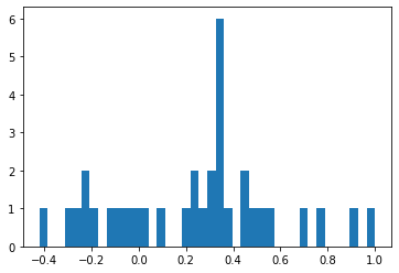

But the most interesting fact for us here concerns the eigenvector $U_2$ associated with the second largest eigenvalue which is also known as the Fiedler vector.

A first result due to Fiedler tells us that the subgraph induced by $G$ on vertices with $U_2(i)\geq 0$ is connected. This is known as Fiedler’s Nodal Domain Theorem (see Chapter 24 in Spectral and Algebraic Graph Theory by Daniel Spielman). We check this fact below both on $U_2$ and $-U_2$ so that here we get a partition of our graph in 2 connected graphs (since we do not have any node $i$ with $U_2(i)=0$).

fiedler = np.array(eigen_vectors[:,-2]).squeeze()
H1 = G.subgraph([i for (i,f) in enumerate(fiedler) if f>=0])
H2 = G.subgraph([i for (i,f) in enumerate(fiedler) if -f>=0])
H = nx.union(H1,H2)
plt.figure(figsize=(7,7))
plt.xticks([])
plt.yticks([])
nx.draw_networkx(H, pos=nx.spring_layout(G, seed=42), with_labels=True)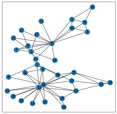

There are many possible partitions of our graph in 2 connected graphs and we see here that the Fiedler vector actually gives a very particular partition corresponding almost exactly to the true communities!

visualize(G, color=[fiedler>=0], cmap="Set2")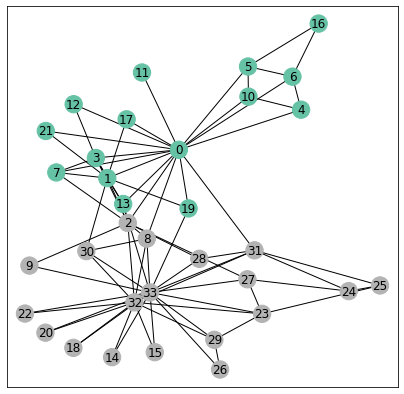

There are actually very few errors made by Fiedler's vector. Another way to see the performance of the Fiedler's vector is to sort its entries and color each dot with its community label as done below:

fiedler_c = np.sort([biclasses,fiedler], axis=1)
fiedler_1 = [v for (c,v) in np.transpose(fiedler_c) if c==1]
l1 = len(fiedler_1)
fiedler_0 = [v for (c,v) in np.transpose(fiedler_c) if c==0]
l0 = len(fiedler_0)
plt.plot(range(l0),fiedler_0,'o',color='red')
plt.plot(range(l0,l1+l0),fiedler_1,'o',color='grey')
plt.plot([0]*35);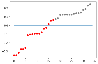

To understand why the partition of Fiedler's vector is so good requires a bit of calculus. To simplify a bit, we will make a small modification about the matrix $S$ and define it to be $S_{ij} = \frac{1}{\sqrt{d_i d_j}}$ if $i\sim j$ or $i=j$ and $S_{ij}=0$ otherwise. We still denote by $\nu_i$ and $U_i$ its eigenvalues and eigenvectors.

Define the (normalized) Laplacian $L=Id-S$ so that the eigenvalues of $L$ are $\lambda_i=1-\nu_i$ associated with the same eigenvector $U_i$ as for $S$. We also define the combinatorial Laplacian $L^* = D-A$.

We then have

$\frac{x^TLx}{x^Tx} = \frac{x^TD^{-1/2}L^* D^{-1/2}x}{x^Tx}\\ = \frac{y^T L^* y}{y^TDy},$

where $y = D^{-1/2}x$. In particular, we get:

$\lambda_2 = 1-\nu_2 = \min_{x\perp U_1}\frac{x^TLx}{x^Tx}\\ = \min_{y\perp d} \frac{y^T L^* y}{y^TDy},$

where $d$ is the vector of degrees.

Rewriting this last equation, we obtain

$\lambda_2 = \min \frac{\sum_{i\sim j}\left(y(i)-y(j)\right)^2}{\sum_i d_i y(i)^2},$

where the minimum is taken over vector $y$ such that $\sum_i d_i y_i =0$.

Now if $y^*$ is a vector achieving the minimum then we get the Fiedler vector (up to a sign) by $U_2 = \frac{D^{1/2}y^*}{\|D^{1/2}y^*\|}$. In particular, we see that the sign of the elements of $U_2$ is the same as the sign of the elements of $y^*$.

To get an intuition about (6), consider the same minimization but with the constraint that $y(i) \in \{-1,1\}$ with the meaning that if $y(i)=1$, then node $i$ is in community $0$ and if $y(i)=-1$ then node $i$ is in community $1$. In this case, we see that the numerator $\sum_{i\sim j}\left(y(i)-y(j)\right)^2$ is the number of edges between the two communities multiplied by 4 and the denominator $\sum_i d_i y(i)^2$ is twice the total number of edges in the graph. Hence the minimization problem is now a combinatorial problem asking for a graph partition $(P_1,P_2)$ of the graph under the constraint that $\sum_{i\in P_1}d_i= \sum_{j\in P_2} d_j$. This last condition is simply saying that the number of edges in the graph induced by $G$ on $P_1$ should be the same as the number of edges in the graph induced by $G$ on $P_2$ (note that this condition might not have a solution). Hence the minimization problem defining $y^*$ in (6) can be seen as a relaxation of this bisection problem. We can then expect the Fiedler vector to be close to this vector of partition $(P_1,P_2)$ at least the signs of its elements which would explain that the partition obtained thanks to the Fiedler vector is balanced and with a small cut, corresponding exactly to our goal here.

So now that we understand the Fiedler vector, we are ready to go back toi GCN. First, we check that the small simplifications made (removing non-linearities...) are really unimportant:

torch.manual_seed(12345)
model = GCN()
W1 = model.conv1.weight.detach().numpy()
W2 = model.conv2.weight.detach().numpy()
W3 = model.conv3.weight.detach().numpy()

iteration = S**3*W1*W2*W3
visualize(torch.tensor(iteration), color=biclasses)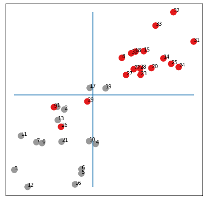

OK, we get (almost) the same embeddings as with the untrained network but we now have a simpler math formula for the output:

$[Y_1,Y_2] = S^3 [R_1, R_2],$

where $R_1,R_2$ are random vectors in $\mathbb{R}^n$ and $Y_1, Y_2$ are the output vectors in $\mathbb{R}^n$ used to do the scatter plot above.

But we can rewrite the matrix $S = \sum_{i}\nu_i U_i U_i^T$ so that we get $S^3 = \sum_{i}\nu_i^3 U_i U_i^T \approx U_1U_1^T + \nu_2^3 U_2U_2^T$ because all others $\nu_i<< \nu_2^3$. Hence, we get

$Y_1 \approx U_1^T R_1 U_1 + \nu_2^3 U_2^T R_1 U_2 \\ Y_2 \approx U_1^T R_2 U_1 + \nu_2^3 U_2^T R_2 U_2$

Recall that the signal about the communities is in the $U_2$ vector so that we can rewrite it more explicitly as

$Y_1(i) \approx a_1 + b_1 U_2(i)\\ Y_2(i) \approx a_2 + b_2 U_2(i),$

where $a_1,a_2,b_1,b_2$ are random numbers of the same magnitude. In other words, the points $(Y_1(i), Y_2(i))$ should be approximately aligned on a line and the two extremes of the corresponding segment should correspond to the 2 communities $U_2(i)\geq 0$ or $U_2(i)\leq 0$.

from sklearn import linear_model
from sklearn.metrics import mean_squared_error
regr = linear_model.LinearRegression()
regr.fit(iteration[:,0].reshape(-1, 1), iteration[:,1])
plt.figure(figsize=(7,7))
plt.xticks([])
plt.yticks([])
h = np.array(iteration)
plt.scatter(h[:, 0], h[:, 1], s=140, c=biclasses, cmap="Set1")
plt.plot(h[:, 0],regr.predict(iteration[:,0].reshape(-1, 1)))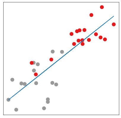

Below, we run a few simulations and compute the mean squared error between the points and the best interpolating line for the random input $[R_1,R_2]$ in blue and for the output $[Y_1, Y_2]$ in orange (that you can hardly see because the error is much smaller). Our theory seems to be nicely validated ;-)

_ = plt.hist(base, bins = 34)
_ = plt.hist(coef, bins = 34)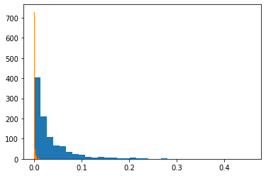

Here we studied a very simple case but more general statements are possible as we will see in a subsequent post. To generalize the analysis made about Fiedler vector requires a little bit of spectral graph theory as explained in the module on spectral Graph Neural Networks, see Deep Learning on graphs (2)

Follow on twitter!

Thanks for reading!