class: center, middle, title-slide count: false # Deep Learning on Graphs<br/> # (2/3) <br/><br/> .bold[Marc Lelarge] .bold[[www.dataflowr.com](https://www.dataflowr.com)] --- # .gray[(1) Node embedding] ## .gray[Language model] ### .gray[one fixed graph, no signal. Ex: community detection] # (2) Signal processing on graphs ## Fourier analysis on graphs ### one fixed graph, various signals. Ex: classification of signals # .gray[(3) Graph embedding] ## .gray[Graph Neural Networks] ### .gray[various graphs. Ex: classification of graphs] --- # Signal processing on graphs ## Fourier analysis on graphs ### one fixed graph, various signals. Ex: classification of signals ## Problem: how to implement a low-pass filter on a graph? We first need to define a notion of frequency domain for graphs. This will allow us to define convolutions on graphs. --- # Recap: Fourier analysis For (smooth) $f:\mathbb{R}^d \to \mathbb{C}$, we define the Fourier transform: $$ \hat{f} (\xi) = \int f(x) e^{-2i\pi x\cdot \xi} dx, $$ so that we have $f(x) = \int \hat{f}(\xi) e^{2i\pi x\cdot \xi} d\xi$. The Fourier transform is a systematic way to decompose ''generic'' functions into a superposition of ''symmetric'' functions. Here, the ''symmetric'' functions are plane waves with frequency $\xi$ defined by $e^{2i\pi x\cdot \xi}$ and can be seen as the eigenfunctions of the Laplacian on $\mathbb{R}^d$: $$ f\mapsto \Delta f = \sum\_{i=1}^d\frac{\partial^2 f}{\partial x\_i^2}. $$ Indeed $\Delta e^{2i\pi x\cdot \xi} = -4\pi^2|\xi|^2 e^{2i\pi x\cdot \xi}$. The Fourier transform allows us to write an arbitrary function as a superposition of eigenfunctions of the Laplacian. This approach works for general graphs! --- # Spectral graph theory For a graph $G=(V,E)$, we denote by $A$ its adjacency matrix and we define its Laplacian by $L=D-A$ where $D = \text{diag}(A 1)$ is the diagonal matrix of (weighted) degrees. -- count: false ## Analogy with $\Delta f = \sum\_{i=1}^d\frac{\partial^2 f}{\partial x\_i^2}$ Recall that $f''(x) \approx \frac{\frac{f(x+h)-f(x)}{h}-\frac{f(x)-f(x-h)}{h}}{h}=\frac{f(x+h)-f(x)+f(x-h)-f(x)}{h^2}$ If $f:V\to \mathbb{R}$, then $$ L f (v) = \sum_{w\sim v} (f(v)-f(w)) $$ --- # Spectral graph theory ## Basics of $L$ We have $v^{T} L v = \sum\_{i < j} A\_{i,j}(v\_i -v\_j)^2$, $L 1=0$ and: let $\lambda\_1=0\leq \lambda\_2\leq ... \leq \lambda\_n$ be the eigenvalues of the Laplacian, then $\lambda\_2>0$ if and only if $G$ is connected. -- count: false ## Fiedler's nodal domain Theorem Let $\lambda\_1=0 < \lambda\_2\leq ... \leq \lambda\_n$ be the eigenvalues of the Laplacian of a connected graph $G$ and let $(u\_1,..., u\_n)$ be the corresponding eigenvectors. For any $k\geq 2$, let $$ W\_k = \\{ i \in V: u_k(i) \geq 0 \\}. $$ Then, the graph induced by $G$ on $W\_k$ has at most $k-1$ connected components. --- .center.width-50[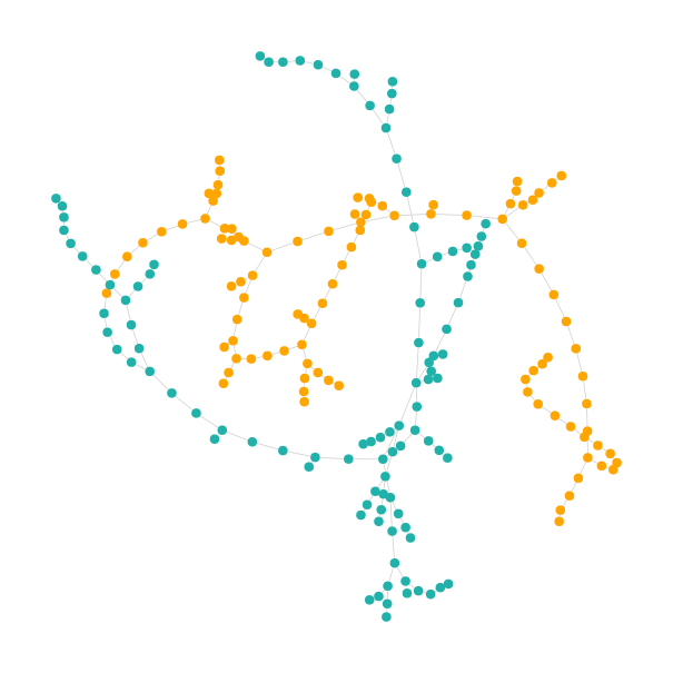] .center[Nodal domain for $\lambda\_2$] --- .center.width-50[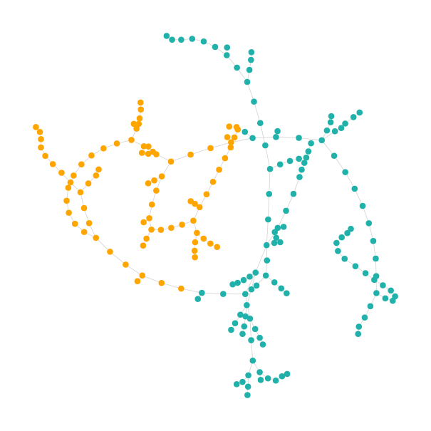] .center[Nodal domain for $\lambda\_3$] --- .center.width-50[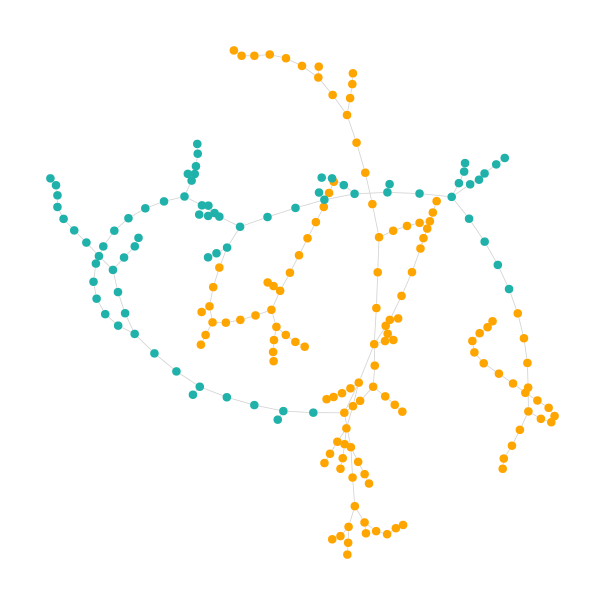] .center[Nodal domain for $\lambda\_4$] --- .center.width-50[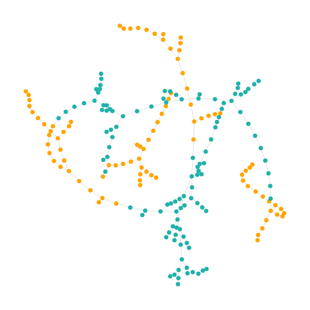] .center[Nodal domain for $\lambda\_6$] --- .center.width-50[] .center[Nodal domain for $\lambda\_{10}$] --- # Graph Fourier transform For a connected graph $G$ with $n$ vertices, we write the spectral decomposition of $L = U\Lambda U^T$, where $$ \Lambda = \text{diag}(\lambda_1=0,\lambda_2,..., \lambda_n), \text{ and } U = (u\_1, ..., u\_n), $$ with $U^TU = U U^T = Id$. For a signal $f\in \mathbb{R}^n$, we define by $\hat{f}(\ell) = u\_{\ell}^T f$ its Fourier mode associated with frequency $\lambda\_{\ell}$. The Fourier transform of $f$ is given by $$ \hat{f} = U^T f, $$ so that we get $$ f = U\hat{f} = \sum\_{\ell} \hat{f}(\ell) u\_{\ell}. $$ --- # Filtering ##convolution = product in spectral domain .center.width-60[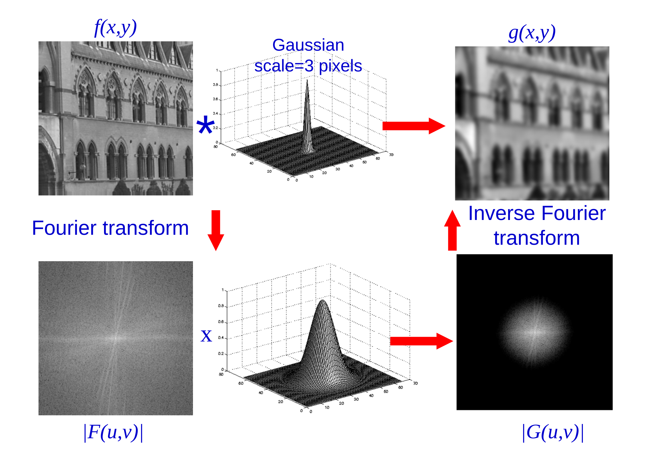] .citation[slide by Andrew Zisserman] --- # Filtering on graphs For a kernel function $k:\mathbb{R}^+ \to \mathbb{R}^+$ acting on the frequency domain, we define the operator $T\_k$ acting on a given signal $f$ as: $$ \widehat{T\_k f}(\ell) = k(\lambda\_{\ell} )\hat{f}(\ell). $$ In matrix form, we write (with $\odot$ the componentwise product): $$ \widehat{T\_k f} = k(\Lambda) \odot \hat{f}. $$ -- count: false Going back in the spatial domain, we get: $$\begin{aligned} T\_k f & = U (k(\Lambda) \odot (U^T f))\\\\ &= U \text{diag}(k(\Lambda)) U^T f \\\\ & = k(L) f. \end{aligned}$$ --- # Learning a localized kernel In order to be able to learn our kernel, we will parametrize them and use polynomial kernels: $$ k\_{\theta}(L) = \sum\_{k=0}^K \theta\_k L^k, $$ where the parameter $\theta\in \mathbb{R}^K$ will be learned. -- count: false Note that if $\text{dist}\_G(i,j)>K$, then we have $(L^K)\_{i,j} =0$, hence our kernel is $K$-localized. Moreover, to compute the output of our filter, we need to evaluate: $$ T\_k f = \sum\_{k=0}^K \theta\_k L^k f. $$ This requires $K$ multiplications by a (sparse) matrix $L$ with a cost $O(K\|E\|)<< n^2$. We defined a .red[convolutional layer for graphs!] --- # Polynomial approximation We are dealing with polynomial kernels. [Wavelets on graphs via spectral graph theory](https://arxiv.org/abs/0912.3848) suggests to use Chebyshev polynomial approximation. The Chebyshev polynomials $T\_k(x)$ are generated by the recurrence: $$ T\_k(x) = 2xT\_{k-1}(x) - T\_{k-2}(x), $$ with $T\_0=1$ and $T\_1=x$. They are an orthogonal basis for $L^2([-1,1],dx/\sqrt{1-x^2})$ so that $$ k(x) = c\_0/2 +\sum\_{k=1}^\infty c\_k T\_k(x), $$ with Chebyshev coefficients $$ c\_k = \frac{2}{\pi} \int\_{-1}^1 \frac{T\_k(x)k(x)}{\sqrt{1-x^2}}dx. $$ --- # Polynomial approximation .center.width-60[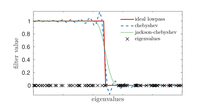] Note: we shift the domain $[-1,1]$ to $[0,\lambda\_{\max}]$ using the transformation $y = \frac{\lambda\_{\max}(x+1)}{2}$. With the shifted Chebyshev polynomials $\overline{T}\_k(y) = T\_k(\frac{2y-\lambda\_{\max}}{\lambda\_{\max}})$, we parametrize the kernel by: $$ k\_\theta(y) = \theta\_0 +\sum\_{k=1}^\infty \theta\_k \overline{T}\_k(y). $$ .citation[source [Fast Eigenspace Approximation using Random Signals](https://arxiv.org/abs/1611.00938)] --- # Convolutional neural networks on graphs The paper [CNN on graphs with fast localized spectral filtering](https://arxiv.org/abs/1606.09375) introduces an additional pooling layer: .center.width-60[] -- count: false ### Performances on MNIST Underlying graph: 8-NN graph of the 2D grid of size $28\times 28$ with weight $W\_{i,j} = e^{-\||z\_i-z\_j\||^2/\sigma^2}$, where $z\_i$ is the 2D coordinate of pixel $i$. .center.width-60[] --- # .gray[(1) Node embedding] ## .gray[Language model] ### .gray[one fixed graph, no signal. Ex: community detection] # (2) Signal processing on graphs ## Fourier analysis on graphs ### one fixed graph, various signals. Ex: classification of signals # .gray[(3) Graph embedding] ## .gray[Graph Neural Networks] ### .gray[various graphs. Ex: classification of graphs] --- class: end-slide, center count: false The end. .bold[[www.dataflowr.com](https://www.dataflowr.com)]